Vector-Quantized Tokenizer Training

StableVQ Practical Guidelines for
Stable Vector-Quantized
Tokenizer Training

A separation-of-concerns framework that turns stable VQ
training from a fragile outcome into a principled property.

Bao Tang1,2,§ Jiahao Guo1,2,§ Haoxiang Cao2,3,§ Wenyu Liu1 Changqian Yu2,† Kun Gai2 Xinggang Wang1,†

1 Huazhong University of Science and Technology 2 KlingAI Research 3 South China Normal University

§ Work done during internship at KlingAI Research. Corresponding authors.

Dynamic STE

Encoder–Decoder

Reliable reconstruction gradients
Region VQ Loss

Codebook

Explicit distribution tracking
Separation
of concerns
Decoupled Schedule

Optimization

Module-specific learning-rate schedules
100%utilization
0new parameters

01 · Motivation

Instability in VQ training

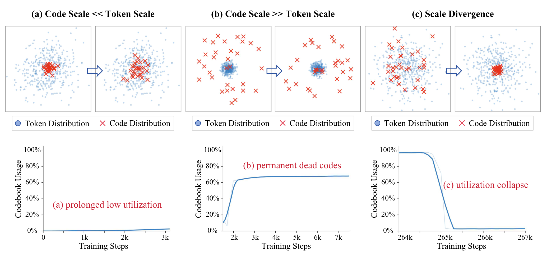
We show three characteristic failure modes encountered during actual VQ training.
The top row illustrates evolving token–code distributions; the bottom row shows their corresponding codebook-usage trajectories.

Three VQ training failure modes caused by changing relationships between token and code distributions

Our perspective · Separation of concerns

One training system. Two distinct responsibilities.

The Encoder–Decoder learns representations for reconstruction under discrete regularization. The Codebook performs distribution alignment. Existing VQ pipelines do not fully separate these objectives: unreliable encoder updates and incomplete codebook learning can destabilize one another.

What does each subsystem need to fulfill its own responsibility?

Encoder–Decoder / Learn the representation

Which gradient should a token trust?

Optimize the task objective while respecting the discrete constraint.

The Encoder receives two signals: an end-task gradient passed through the STE, and a commitment gradient pulling tokens toward their assigned codes. Their balance is critical as both distributions evolve.

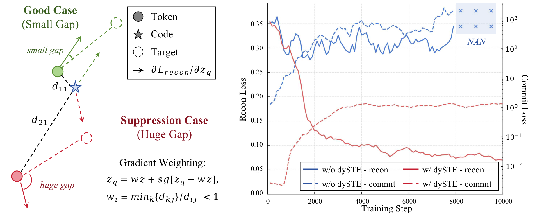
But the end-task gradient is evaluated at the code, not at the token. When the pair is far apart, a useful direction for the code can be misleading for the token—even pushing it away from its assigned code, against the commitment signal.

The mismatch can then reinforce itself: unreliable gradients pull the distributions further apart, making subsequent estimates worse. This feedback can ultimately cause extremely low codebook utilization or even NaN values; the Scale Divergence described above is one example.

Make gradient trust distance-aware. Attenuate the STE-passed end-task gradient for relatively distant token–code assignments.

Dynamic STE
Codebook / Track the distribution

Where should an unused code go?

Fit the code distribution to the evolving token distribution.

In conventional VQ training, the Codebook receives only one learning signal—the VQ loss—but this signal has two limitations:

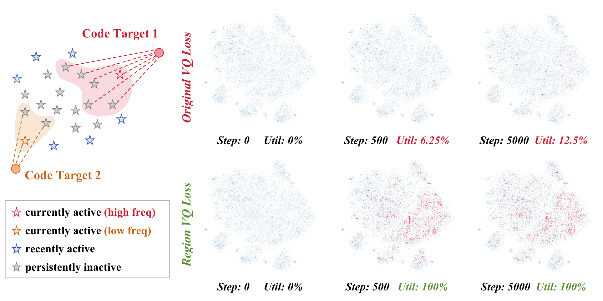
  1. Missing targets. Only selected codes receive direct supervision; when utilization is low, most codes receive no learning signal.
  2. Unused allocation information. Hit frequency affects the update magnitude of selected codes, but is not translated into guidance for the distribution of the Codebook as a whole.

Shared projectors spread gradients to inactive codes, but do not assign them explicit targets. Their activation can still depend on incidental movement rather than directed learning. Making a code move is not the same as telling it where to go.

Turn frequency into allocation. Propagate targets to inactive codes in proportion to hit frequency, providing dense and directed learning signals.

Region VQ Loss

Joint optimization / Respect both objectives

Different responsibilities.
Why the same schedule?

Decoupled Schedule

Once each subsystem has an appropriate learning signal, we revisit how they learn together. Warmup and annealing help the Encoder–Decoder balance its complex objectives. The Codebook has a cleaner task: continuously track a changing distribution.

Making the Codebook follow the same schedule can unnecessarily slow that tracking, especially early in training. We therefore study the schedules independently: retain warmup and annealing for the Encoder–Decoder, and sustain a sufficiently high learning rate for the Codebook.

Separate the objectives first. Then give each the optimization dynamics it needs.

02 · Method

Isolate the cause. Test the intervention.

Three lightweight, parameter-free components follow from this separation. Controlled pilot studies test each premise:
freeze one subsystem to examine the other, then vary their schedules independently.

01

For the Encoder–Decoder

Dynamic STE

Use the closest token in the batch as a reference for each code. Weight a token’s STE gradient by the reference squared distance divided by its own squared distance to that code. The best match retains its full gradient; relatively distant assignments are attenuated.

  • No threshold hyperparameter
  • Attenuates unreliable gradients
  • Only changes the magnitude of the backward signal
Dynamic STE design and controlled training-loss comparison

Pilot study / Isolate the Encoder–Decoder

Can training fail even when the Codebook stays fixed?

Controlled setup
Freeze the Codebook and train only the Encoder–Decoder. Compare standard STE with Dynamic STE, tracking reconstruction and commitment losses.
Observed result
Standard STE produces commitment-loss spikes and reconstruction oscillations, eventually reaching NaN. Dynamic STE keeps commitment loss controlled while reconstruction loss falls.
What this isolates
Codebook motion is not required for instability. The gradient estimation gap can destabilize Encoder training on its own.
02

For the Codebook

Region VQ Loss

Active codes propagate their token-mean targets to nearby persistently inactive codes, with quotas proportional to hit frequency. A FIFO activity window protects recently active codes; overlapping recipients average the targets they receive.

  • Dense, localized and directed supervision
  • Distribution-aware code allocation
  • More inactive codes directed toward higher token mass
Region VQ target propagation and codebook distribution alignment over training

Pilot study / Isolate the Codebook

Can the Codebook align without help from a moving Encoder?

Controlled setup
Freeze the Encoder and train only the Codebook, using an expressive two-layer ViT shared projector. Visualize tokens and codes at steps 0, 500, and 5,000.
Observed result
Standard VQ loss reaches only 12.5% utilization at 5,000 steps. Region VQ reaches 100% by step 500 and maintains it.
What this isolates
A shared projector alone does not supply the missing objective. Directed targets let the Codebook align without relying on Encoder fluctuations to activate codes.
03

For system-level optimization

Decoupled Schedule

Use separate learning-rate schedules for the two subsystems: the Encoder–Decoder uses warmup & annealing, while the Codebook uses a sufficiently high constant rate to track evolving tokens from the first step.

  • Warmup + annealing for reconstruction
  • Sustained learning rate for distribution tracking
  • No additional forward or backward operation
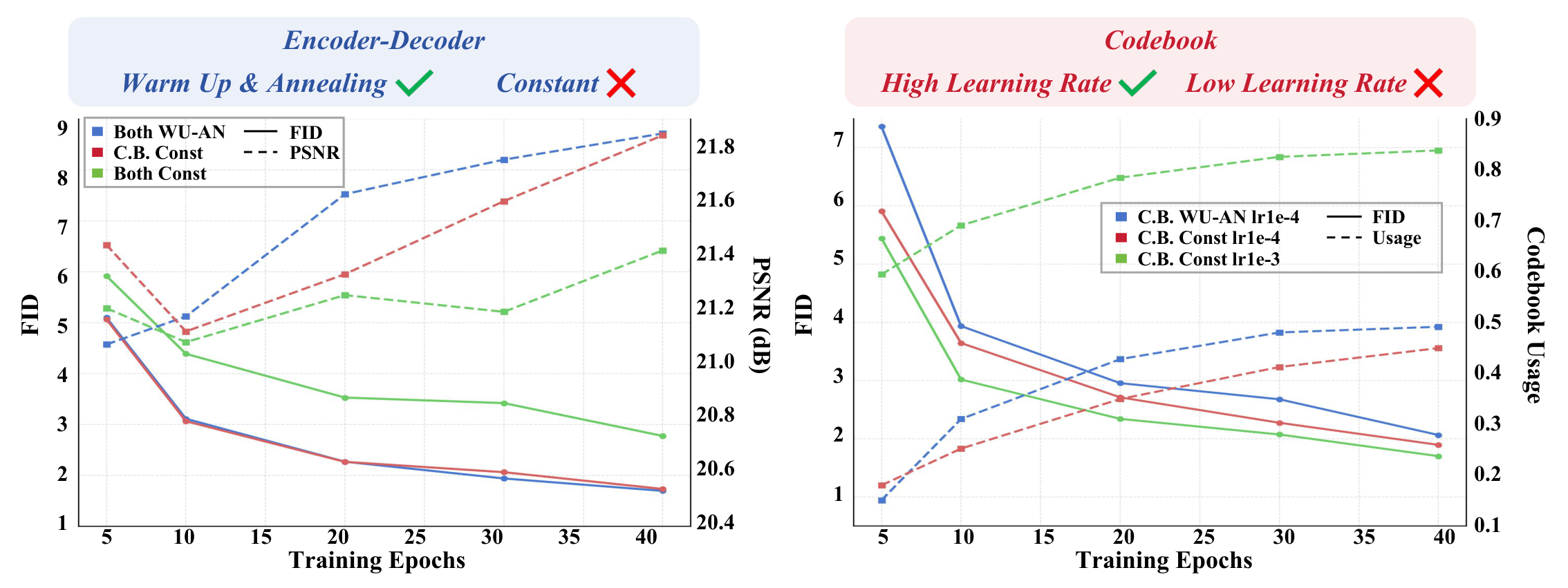
Controlled study of learning-rate schedules for the encoder-decoder and codebook

Pilot study / Separate the schedules

Which subsystem actually needs warmup and annealing?

Left · FVQ architecture
Vary which module uses warmup and annealing. A constant Codebook rate preserves reconstruction quality; making the Encoder–Decoder constant-rate as well causes a clear quality drop.
Right · SimVQ architecture
Compare Codebook warmup-and-annealing at 10−4 with constant rates of 10−4 and 10−3. The higher constant rate yields substantially better utilization—not merely a change in schedule shape.

The two subsystems benefit from different optimization dynamics: scheduled convergence for representation learning, sustained updates for distribution tracking.

03 · Component ablations

Why each component matters

Two opposing distribution mismatches expose complementary optimization needs:
stable encoder gradients, explicit codebook targets, and fast distribution tracking.

Ablation 01 / Expansion

Stability and code coverage need to improve together

Small-range initialization · Linear-1 projector. The baseline uses warmup and annealing with a peak learning rate of 10−4;
Decoupled Schedule gives the codebook a constant 10−3 learning rate.

Region VQDyn. STEDe. Sch.Peak Commit.Usage ↑rFID ↓LPIPS ↓PSNR ↑SSIM ↑
53.1149.13%2.060.229721.650.5730
<0.11.27%6.680.310019.890.5026
<0.183.77%1.710.220921.790.5864
<0.121.66%2.070.235421.360.5665
<0.1100%1.720.220021.840.5854
<0.1100%1.750.220621.850.5860
<0.1100%1.700.220821.810.5879

✓ component enabled · Dyn. STE: Dynamic STE · De. Sch.: Decoupled Schedule · Peak Commit.: peak commitment loss. Bold marks the best value in each metric.

Dynamic STE controls commitment-loss spikes; low usage reveals conventional VQ’s reliance on Encoder fluctuations.

Decoupled Schedule improves tracking and raises usage to 83.77%, while standard VQ still leaves codes inactive.

Region VQ Loss recovers 100% usage with either component; alone, slow codebook updates under warmup lead to NaN collapse.

Together, all three components achieve 100% utilization and 1.70 rFID, combining stable gradients, dense supervision, and sustained tracking.

Ablation 02 / Shrinkage

Inactive codes need explicit learning targets

1024-dimensional codebook · ViTBlock-2 projector. With ℓ₂ normalization, codes are broadly distributed while image tokens concentrate in a smaller region.

ProjectorRegion VQInitializationUsage ↑rFID ↓PSNR ↑SSIM ↑LPIPS ↓
ViTBlock-2Uniform18.75%2.435520.97890.56770.2414
ViTBlock-2Gaussian62.50%1.953021.37740.58360.2273
ViTBlock-2Uniform100%1.817621.54970.58960.2210
ViTBlock-2Gaussian100%1.896621.46030.59310.2255

Region VQ restores 100% utilization under both initializations and improves reconstruction across all metrics, with the strong shared projector used in FVQ.

04 · Robustness analysis

Testing across a broader range of configurations

Continuous sweeps test sensitivity to initialization, projector design, and learning rate.
Usage-recovery experiments then evaluate the full method under evolving token–code mismatch.

Appendix D.1–D.2 / Initialization & shared projectors

Initialization and projector sensitivity

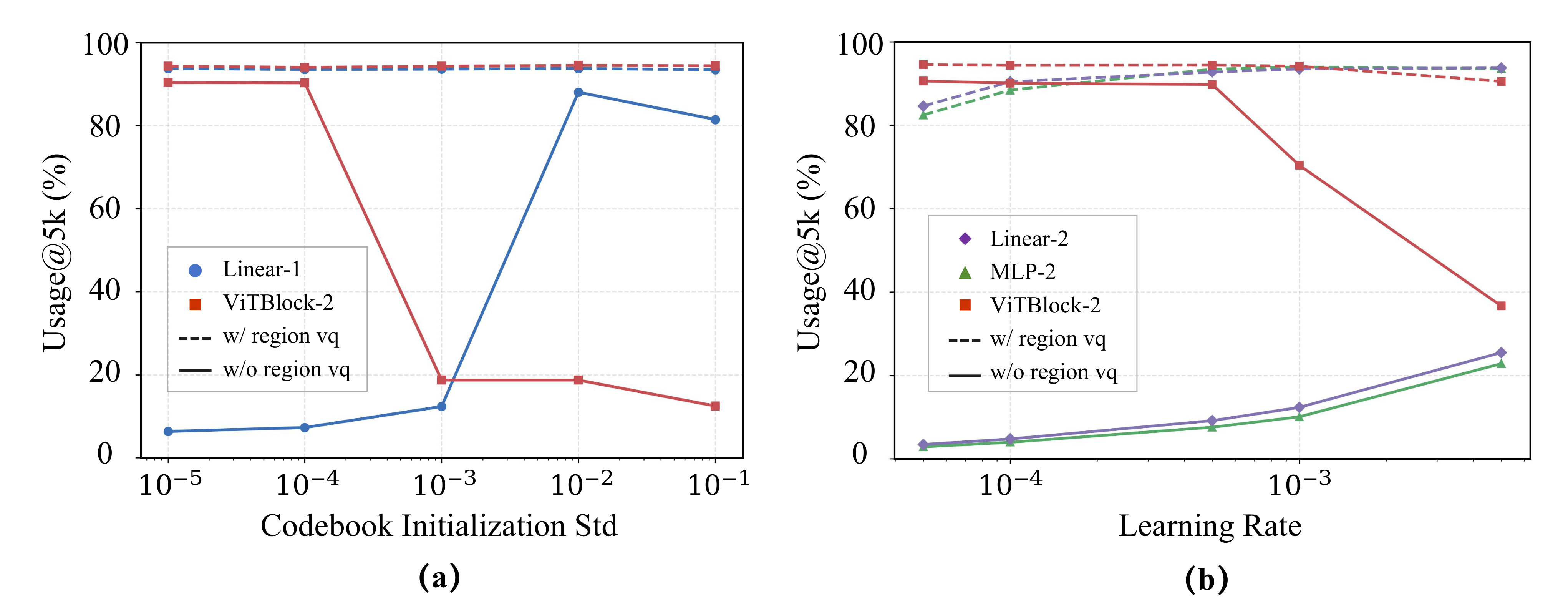
Controlled setting Frozen Encoder · fixed target distribution · utilization at 5K steps · 65,536-token measurement window

Combined analysis figure: (a) Usage at 5K steps across Gaussian initialization scales for Linear-1 and ViTBlock-2; (b) Usage at 5K steps across learning rates for Linear-2, MLP-2, and ViTBlock-2, comparing standard VQ loss with Region VQ Loss

(a) Initialization scale · D.1

Vary the Gaussian standard deviation from 10−5 to 10−1 with Linear-1 and ViTBlock-2 shared projectors. Small scales slow recovery with Linear-1; larger scales leave many codes inactive with ViTBlock-2.

Region VQ keeps both near full utilization across the tested scales.

(b) Projector & learning rate · D.2

Fix the Gaussian initialization scale at 10−4 and vary the learning rate for Linear-2, MLP-2, and ViTBlock-2. Linear and MLP projectors recover slowly; ViTBlock-2 loses usage at large learning rates.

Region VQ broadens the usable learning-rate range across all three designs.

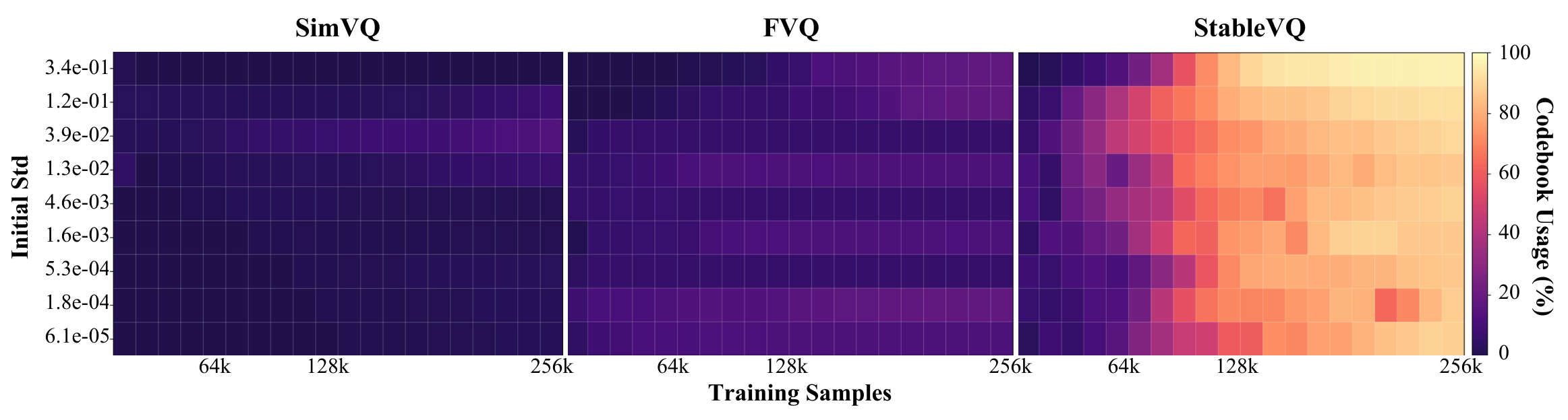
Codebook usage recovery heatmaps for SimVQ, FVQ and StableVQ
Usage recovery. StableVQ rapidly restores high codebook usage across a broad range of initialization scales.

Robustness under mismatch

Recovery across distribution mismatch

Each heatmap row tests a different initial token–code relationship. StableVQ recovers usage across a broad range of mismatch settings.
Usage Recovery AUC summarizes the usage trajectories across these settings; higher is better.

SimVQ2.17 UR-AUC FVQ8.08 UR-AUC StableVQ60.59 UR-AUC

05 · Reconstruction & generation

Stable training, strong visual tokens

On ImageNet 256×256, StableVQ combines full codebook utilization with strong reconstruction and competitive downstream class-conditional generation.

Codebook usage 100%

for both 16K and 262K codebooks

Reconstruction · 16K 1.13

rFID · 120 epochs

Reconstruction · 262K 0.92

rFID · 120 epochs

Generation FID 2.18

ImageNet 256×256 with IBQ-L generator

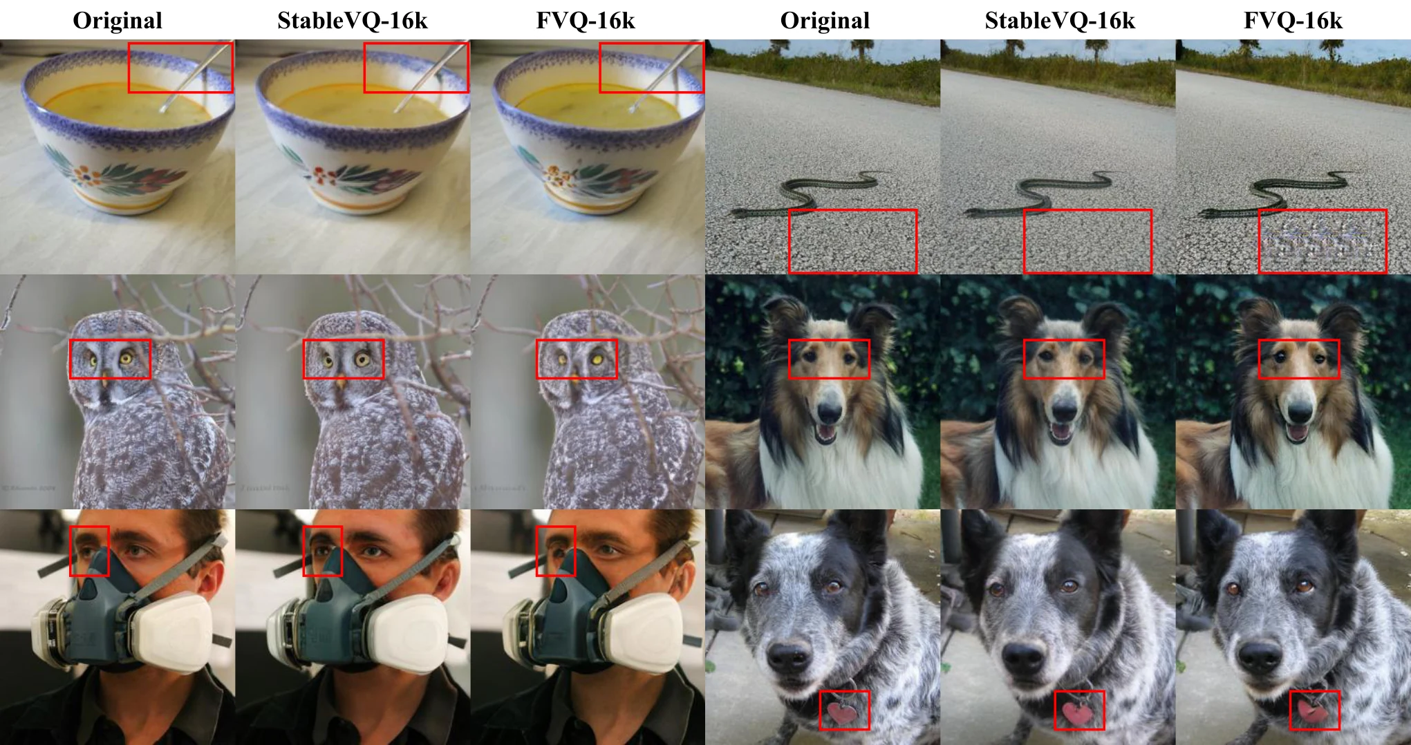
Selected reconstruction results

ImageNet 256×256 · 16×16 tokens
MethodProjectorEpochsCodebookrFID ↓LPIPS ↓Usage ↑
SimVQLinear-14016K × 2562.890.2492100%
FVQViTBlock-24016K × 2561.700.2176100%
StableVQLinear-14016K × 2561.220.2235100%
StableVQLinear-112016K × 2561.130.2134100%
StableVQLinear-1120262K × 2560.920.1893100%

07 · Citation

Build on StableVQ

If StableVQ is useful for your research, please consider citing our work.

Questions: X. Wang · C. Yu

BibTeX
@misc{tang2026stablevq,
  title={StableVQ: Practical Guidelines for Stable Vector-Quantized Tokenizer Training},
  author={Bao Tang and Jiahao Guo and Haoxiang Cao and Wenyu Liu and Changqian Yu and Kun Gai and Xinggang Wang},
  year={2026},
  eprint={2609.26774},
  archivePrefix={arXiv},
  primaryClass={cs.CV},
  url={https://arxiv.org/abs/2609.26774},
}